hvPlot-Beispiele#

Installation#

Um die Beispiele ausführen zu können, muss zusätzlich Snappy installiert werden.

Mit Spack könnt ihr Snappy in eurem Kernel bereitstellen, z.B. mit:

$ spack env activate python-311
$ spack install snappy

Alternativ könnt ihr Snappy auch mit anderen Paketmanagern installieren, z.B.

Für Debian/Ubuntu:
```
$ sudo apt install libsnappy-dev
```
Für Windows:

Snappy benötigt Microsoft Visual C++ ≥ 14.0. Dies kann installiert werden mit den Microsoft C++ Build Tools.
Für Mac OS:
```
$ brew install snappy
```

Anschließend sollten für euren Kernel noch weitere Pakete installiert werden, z.B. mit:

$ pipenv install intake intake-parquet s3fs python-snappy pyviz-comms
…

Einführung#

Als erstes importieren wir NumPy und pandas um anschließend einen kleinen Satz zufälliger Daten zu erstellen:

[1]:

import numpy as np
import pandas as pd


index = pd.date_range("1/1/2000", periods=1000)
df = pd.DataFrame(
    np.random.randn(1000, 4), index=index, columns=list("ABCD")
).cumsum()

df.head()

[1]:

	A	B	C	D
2000-01-01	1.431985	1.378913	0.539567	0.257977
2000-01-02	1.266573	0.834050	1.176750	1.458363
2000-01-03	1.799283	0.945437	1.792629	-0.220764
2000-01-04	2.131248	0.160377	1.186063	-0.702810
2000-01-05	3.574972	2.274926	1.759324	-1.297244

pandas`.plot ()`-API#

pandas bietet standardmäßig Matplotlib-basiertes Plotten mit der .plot()-Methode:

[2]:

%matplotlib inline

df.plot();

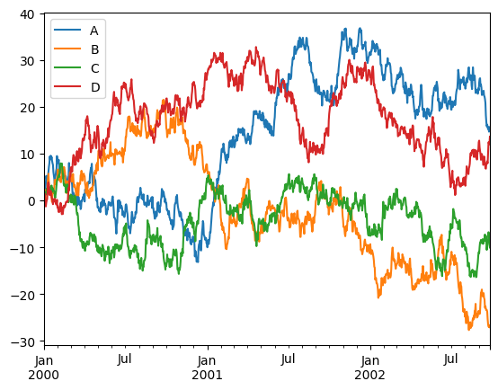
../../../../_images/bokeh_integration_holoviews_hvplot_examples_5_0.png

Das Ergebnis ist ein PNG-Bild, das leicht angezeigt werden kann, ansonsten aber statisch ist.

Hinweis: In pandas > 0.25.0 kann das Backend ausgetauscht werden, z.B. mit pd.options.backend.plotting == 'holoviews',. Weitere Informationen hierzu findet ihr unter pandas-API.

`.hvplot()`#

Wenn wir statt %matplotlib inline zu import hvplot.pandas und der df.hvplot-Methode wechseln, , wird jetzt ein interaktiv erforschbares Bokeh-Diagramm erzeugt mit Verschieben und Vergrößern/Verkleinern sowie anklickbaren Legenden:

[3]:

import hvplot.pandas

df.hvplot()

[3]:

Ein solches interaktive Diagramm erleichtert das Erkunden der der Daten erheblich, ohne dass hierfür zusätzlicher Code geschrieben werden müsste.

Native `hvPlot`-API#

Für das obige Diagramm hat hvPlot die pandas-.hvplot()-Methode dynamisch hinzugefügt, sodass ihr dieselbe Syntax wie bei pandas-Plots verwenden könnt. Wenn ihr ein expliziteres Vorgehen bevorzugt, könnt ihr stattdessen direkt mit den hvPlot-Objekten arbeiten:

[4]:

import holoviews as hv

from hvplot import hvPlot

hv.extension("bokeh")

plot = hvPlot(df)
plot(y=["A", "B", "C", "D"])

[4]:

Hilfe#

Wenn ihr in IPython oder Jupyter-Notebooks arbeitet, vervollständigen die hvplot-Methoden automatisch gültige Schlüsselwörter. Wenn ihr beispielsweise nach dem Deklarieren des Plottyps die Tabulatortaste drücken, werden alle gültigen Schlüsselwörter und die Dokumentzeichenfolge angezeigt:

df.hvplot.line(TAB

Außerhalb einer interaktiven Umgebung werden mit hvplot.help alle Informationen für einen Diagrammtyp angezeigt, z.B.:

[ ]:

hvplot.help("line")

Siehe auch:

Weitere Informationen zu den verfügbaren Optionen erhaltet ihr in Customization.

Plotting#

In den folgenden Beispielen wird neben der pandas- auch die dask-hvPlot-API verwendet:

[6]:

import hvplot.dask

Das hvplot.sample_data-Modul erstellt diese Datensätze als Intake-Datenkataloge, die wir mit pandas laden können:

[7]:

from hvplot.sample_data import airline_flights, us_crime


crime = us_crime.read()
print(type(crime))
crime.head()

<class 'pandas.core.frame.DataFrame'>

[7]:

	Year	Population	Violent crime total	Murder and nonnegligent Manslaughter	Legacy rape /1	Revised rape /2	Robbery	Aggravated assault	Property crime total	Burglary	...	Violent Crime rate	Murder and nonnegligent manslaughter rate	Legacy rape rate /1	Revised rape rate /2	Robbery rate	Aggravated assault rate	Property crime rate	Burglary rate	Larceny-theft rate	Motor vehicle theft rate
0	1960	179323175	288460	9110	17190	NaN	107840	154320	3095700	912100	...	160.9	5.1	9.6	NaN	60.1	86.1	1726.3	508.6	1034.7	183.0
1	1961	182992000	289390	8740	17220	NaN	106670	156760	3198600	949600	...	158.1	4.8	9.4	NaN	58.3	85.7	1747.9	518.9	1045.4	183.6
2	1962	185771000	301510	8530	17550	NaN	110860	164570	3450700	994300	...	162.3	4.6	9.4	NaN	59.7	88.6	1857.5	535.2	1124.8	197.4
3	1963	188483000	316970	8640	17650	NaN	116470	174210	3792500	1086400	...	168.2	4.6	9.4	NaN	61.8	92.4	2012.1	576.4	1219.1	216.6
4	1964	191141000	364220	9360	21420	NaN	130390	203050	4200400	1213200	...	190.6	4.9	11.2	NaN	68.2	106.2	2197.5	634.7	1315.5	247.4

5 rows × 22 columns

Alternativ können wir dask.DataFrame verwenden:

[8]:

flights = airline_flights.to_dask().persist()
print(type(flights))
flights.head()

<class 'dask.dataframe.core.DataFrame'>

[8]:

	year	month	day	dayofweek	dep_time	crs_dep_time	arr_time	crs_arr_time	carrier	flight_num	...	taxi_in	taxi_out	cancellation_code	carrier_delay	weather_delay	nas_delay	security_delay	late_aircraft_delay
0	2008.0	11.0	15.0	6.0	1411.0	1420.0	1535.0	1546.0	b'OO'	4391.0	...	5.0	11.0	None	NaN	NaN	NaN	NaN	NaN
1	2008.0	11.0	28.0	5.0	1222.0	1230.0	1345.0	1356.0	b'OO'	4391.0	...	5.0	15.0	None	NaN	NaN	NaN	NaN	NaN
2	2008.0	11.0	22.0	6.0	1414.0	1420.0	1540.0	1546.0	b'OO'	4391.0	...	5.0	10.0	None	NaN	NaN	NaN	NaN	NaN
3	2008.0	11.0	15.0	6.0	1304.0	1305.0	1507.0	1519.0	b'OO'	4392.0	...	10.0	9.0	None	NaN	NaN	NaN	NaN	NaN
4	2008.0	11.0	22.0	6.0	1323.0	1305.0	1536.0	1519.0	b'OO'	4392.0	...	5.0	21.0	None	0.0	0.0	0.0	0.0	17.0

5 rows × 29 columns

Die Plot-API#

Die Schnittstellen

dask.dataframe.DataFrame.hvplot
pandas.DataFrame.hvplot
intake.DataSource.plot

und ihre Series-Äquivalente bieten eine leistungsfähige High-Level-API um auch komplexe Plots erzeugen zu können. Dabei kann die .hvplot-API entweder direkt oder als Namespace verwendet werden, um bestimmte Plottypen zu generieren.

Die expliziteste Methode zur Verwendung der Plot-API besteht darin, die Namen der Spalten anzugeben, die auf der x- bzw. y-Achse geplottet werden sollen:

[9]:

crime.hvplot.line(x="Year", y="Violent Crime rate")

[9]:

Zusätzlich kann auch noch der Diagrammtyp mit kind angegeben werden:

[10]:

crime.hvplot(x="Year", y="Violent Crime rate", kind="scatter")

[10]:

Mit der by-Variable könnt ihr die Daten in einer oder mehreren zusätzlichen Spalten gruppieren. Als Beispiel wird im Folgenden die Abfahrtsverzögerung ('depdelay') als Funktion der 'distance' dargestellt und die Daten nach 'carrier' gruppiert:

[11]:

flight_subset = flights[flights.carrier.isin([b"OH", b"F9"])]
flight_subset.hvplot(
    x="distance",
    y="depdelay",
    by="carrier",
    kind="scatter",
    alpha=0.2,
    persist=True,
)

[11]:

Im obigen Beispiel haben wir die x- und y-Achsen explizit angegeben.

Andernfalls würde für die x-Achse die pandas-Indexspalte verwendet werden und für die y-Achse alle Nicht-Index-Spalten mit der Standardbezeichnung 'value'. Wollt ihr nur die y-Achsenbezeichnung explizit angeben, so steht euch die value_label-Option zur Verfügung.

[12]:

crime.hvplot(
    x="Year",
    y=["Violent Crime rate", "Robbery rate", "Burglary rate"],
    value_label="Rate (per 100k people)",
)

[12]:

Der `hvplot`-Namespace#

Statt des kind-Argument können wir auch den hvplot-Namespace für den Plotaufruf zu verwenden. Die unterstützten Plottypen lassen sich leicht ermitteln mit der Tab-Vervollständigung, also

crime.hvplot.TAB

Verfügbare Diagrammtypen sind:

area() zeichnet ein Flächendiagramm ähnlich einem Liniendiagramm, außer dass der Bereich unter der Kurve gefüllt und optional gestapelt wird
bar() zeichnet ein Flächendiagramm ähnlich einem Liniendiagramm, außer dass der Bereich unter der Kurve gefüllt und optional gestapelt wird
bivariate() zeichnet ein Flächendiagramm ähnlich einem Liniendiagramm, außer dass der Bereich unter der Kurve gefüllt und optional gestapelt wird
box() zeichnet ein Box-Whisker-Diagramm, in dem die Verteilung einer oder mehrerer Variablen verglichen wird
heatmap() zeichnet Hex-Bins
hexbins() zeichnet die Verteilung eines oder mehrerer Histogramme als Satz von Containern
histogram() zeichnet die Kernel-Dichteschätzung einer oder mehrerer Variablen
kde() zeichnet die Kernel-Dichteschätzung einer oder mehrerer Variablen
line() zeichnet ein Liniendiagramm (z.B. für eine Zeitreihe)
step() zeichnet ein Schrittdiagramm, das einem Liniendiagramm ähnelt
scatter() zeichnet ein Streudiagramm, in dem zwei Variablen verglichen werden
table() erzeugt eine SlickGrid-Datentabelle
violin() zeichnet ein Violinen-Diagramm, in dem die Verteilung einer oder mehrerer Variablen mithilfe der Kernel-Dichteschätzung verglichen wird

`area()`#

Wie die meisten anderen Diagrammtypen unterstützt das area-Diagramm die drei oben beschriebenen Möglichkeiten zum Definieren eines Diagramms. Ein Flächendiagramm ist am nützlichsten, wenn mehrere Variablen in einem gestapelten Diagramm dargestellt werden. Dies kann durch Angabe für die x-, y- und by-Spalten erreicht werden oder mit columns und index/use_index als Optionen für die x-Achse.

[13]:

crime.hvplot.area(x="Year", y=["Robbery", "Aggravated assault"])

[13]:

Wir können auch explizit stacked auf False setzen und einen alpha-Wert definieren und um die Werte direkt vergleichen zu können:

[14]:

crime.hvplot.area(
    x="Year", y=["Aggravated assault", "Robbery"], stacked=False, alpha=0.4
)

[14]:

Eine andere Verwendung für ein Flächendiagramm besteht darin, die Streuung eines Werts zu visualisieren. Wenn wir beispielsweise den Flugdatensatz verwenden, möchten wir möglicherweise die Streuung der mittleren Verspätungswerte zwischen den Fluggesellschaften sehen. Zu diesem Zweck berechnen wir die mittlere Verzögerung nach Tag und Carrier und dann die minimale/maximale mittlere Verzögerung für alle Carrier. Da die Ausgabe von hvplot nur ein reguläres Holoviews-Objekt ist, können wir den Overlay-Operator (*) verwenden, um die Diagramme übereinander zu platzieren.

[15]:

delay_min_max = (
    flights.groupby(["day", "carrier"])["carrier_delay"]
    .mean()
    .groupby("day")
    .agg([np.min, np.max])
)
delay_mean = flights.groupby("day")["carrier_delay"].mean()

delay_min_max.hvplot.area(
    x="day", y="amin", y2="amax", alpha=0.2
) * delay_mean.hvplot()

[15]:

`bar()`#

Im einfachsten Fall können wir .hvplot.bar verwenden. Um die Beschriftung auf der x-Achse um 90° zu drehen, geben wir noch rot=90 an.

[16]:

crime.hvplot.bar(x="Year", y="Violent Crime rate", rot=90)

[16]:

Wenn wir stattdessen mehrere Spalten vergleichen möchten, können wir eine Liste von Spalten festlegen. Mit der stacked-Option können wir dann die Spaltenwerte einfacher vergleichen:

[17]:

crime.hvplot.bar(
    x="Year",
    y=["Violent crime total", "Property crime total"],
    stacked=True,
    rot=90,
    width=800,
    legend="top_left",
)

[17]:

`scatter()`#

Das Streudiagramm unterstützt viele der Funktionen der obigen Diagrammtypen, kann jedoch mit der c-Option auch eingefärbt werden.

[18]:

crime.hvplot.scatter(x="Violent Crime rate", y="Burglary rate", c="Year")

[18]:

Um Farbe zur Darstellung einer Dimension zu verwenden, kann die cmap-Option genutzt werden werden, um die zu verwendende Farbkarte anzugeben. Zusätzlich kann die Farbleiste deaktiviert werden mit colorbar=False.

`step()`#

Ein Schrittdiagramm ist einem Liniendiagramm sehr ähnlich, aber anstatt linear zwischen Abtastwerten zu interpolieren, visualisiert das Schrittdiagramm diskrete Schritte. Die Position der Schritte kann mit dem where-Schlüsselwort un den Werten 'pre', 'mid' (Standard) und 'post' gesteuert werden.

[19]:

crime.hvplot.step(x="Year", y=["Robbery", "Aggravated assault"])

[19]:

`hexbin()`#

Mit der hexbin-Methode können Sie hexagonale Bin-Diagramme erstellen. Sie können eine nützliche Alternative zu Streudiagrammen sein, wenn die Daten zu dicht sind, um jeden Punkt einzeln zu zeichnen. Da unsere Flugdaten nicht gleichmäßig auf einer linearen Skala verteilt sind, verwenden wir die logz-Option für eine logarithmische Skala.

[20]:

flights.hvplot.hexbin(
    x="airtime", y="arrdelay", width=600, height=500, logz=True
)

[20]:

`bivariate()`#

Mit der bivariate-Methode könnt ihr ein 2D-Dichtediagramm erstellen. Bivariate Diagramme sind neben Hexbin-Diagrammen eine weitere Alternative zu Streudiagrammen, wenn die Daten zu dicht sind, um jeden Punkt einzeln zu zeichnen.

[21]:

crime.hvplot.bivariate(
    x="Violent Crime rate", y="Burglary rate", width=600, height=500
)

[21]:

`heatmap()`#

HeatMap kann die Beziehung zwischen drei Variablen anzeigen und neben den Variablen 'x' und 'y' zusätzlich 'C' anzeigen. Zusätzlich werden mit der reduce_function die Werte für jeden Container aus den Stichproben berechnet.

[22]:

flights.compute().hvplot.heatmap(
    x="day", y="carrier", C="depdelay", reduce_function=np.mean, colorbar=True
)

[22]:

`table()`#

Im Gegensatz zu allen anderen Plottypen kann für eine Tabelle nur angegeben werden, ob alle Spalten oder mit columns nur eine Teilmenge angezeigt werden soll.

[23]:

crime.hvplot.table(
    columns=["Year", "Population", "Violent Crime rate"], width=400
)

[23]:

`hist()`#

Das Zeichnen von Verteilungen unterscheidet sich geringfügig von anderen Plots, da sie im einfachen Fall nur eine Variable darstellen. Daher muss bei diesem Plottyp kein index oder x-Wert angegeben werden, sondern

deklariert eine einzelne y-Variable, z.B. source.plot.hist(variable) oder
deklariert eine y-Variable und eine by-Variable, z.B. source.plot.hist(variable, by='Group') oder
deklariert Spalten oder zeichnet alle Spalten, z.B. source.plot.hist() oder source.plot.hist(columns=['A', 'B', 'C'])

[24]:

crime.hvplot.hist(y="Violent Crime rate")

[24]:

Alternativ önnen wir auch die Verteilung mehrerer Spalten darstellen:

[25]:

columns = ["Violent Crime rate", "Property crime rate", "Burglary rate"]
crime.hvplot.hist(y=columns, bins=50, alpha=0.5, legend="top", height=400)

[25]:

Wir können die Daten auch nach anderen Variablen gruppieren und die Carrier in eigene subplots aufteilen:

[26]:

flight_subset = flights[flights.carrier.isin([b"AA", b"US", b"OH"])]
flight_subset.hvplot.hist(
    "depdelay",
    by="carrier",
    bins=20,
    bin_range=(-20, 100),
    width=300,
    subplots=True,
)

[26]:

`kde()`, `density()`#

Ihr könnt Dichtediagramme auch mit hvplot.kde() oder hvplot.density() erstellen:

[27]:

crime.hvplot.kde(y="Violent Crime rate")

[27]:

Der Vergleich der Verteilung mehrerer Spalten ist ebenfalls möglich:

[28]:

columns = ["Violent Crime rate", "Property crime rate", "Burglary rate"]
crime.hvplot.kde(y=columns, alpha=0.5, value_label="Rate", legend="top_right")

[28]:

hvplot.kde unterstützt auch das by-Schlüsselwort:

[29]:

flight_subset = flights[flights.carrier.isin([b"AA", b"US", b"OH"])]
flight_subset.hvplot.kde(
    "depdelay", by="carrier", xlim=(-20, 70), width=300, subplots=True
)

[29]:

`box()`#

Genau wie die anderen verteilungsbasierten Diagrammtypen unterstützt das Box-Whisker-Diagramm das Zeichnen einer einzelnen Spalte:

[30]:

crime.hvplot.box(y="Violent Crime rate")

[30]:

Es unterstützt auch mehrere Spalten und die gleichen Optionen wie berits oben genannt:legend, invert und value_label:

[31]:

columns = [
    "Burglary rate",
    "Larceny-theft rate",
    "Motor vehicle theft rate",
    "Property crime rate",
    "Violent Crime rate",
]
crime.hvplot.box(
    y=columns,
    group_label="Crime",
    legend=False,
    value_label="Rate (per 100k)",
    invert=True,
)

[31]:

Auch die Verwendung des by-Schlüsselworts zum Aufteilen der Daten in mehrere Teilmengen wird unterstützt:

[32]:

flight_subset = flights[flights.carrier.isin([b"AA", b"US", b"OH"])]
flight_subset.hvplot.box("depdelay", by="carrier", ylim=(-10, 70))

[32]:

Zusammengesetzte Diagramme#

Eine der Hauptstärken von HoloViews ist die einfache Erstellung verschiedener Diagramme. Einzelne Diagramme können mit den Operatoren * und + überlagert bzw. zusammengesetzt werden.

Siehe auch:

Composing Elements

[33]:

crime.hvplot(x="Year", y="Violent Crime rate") * crime.hvplot.scatter(
    x="Year", y="Violent Crime rate", c="k"
)

[33]:

Wir können auch verschiedene Diagramme und Tabellen zusammen erstellen:

[34]:

(
    crime.hvplot.bar(x="Year", y="Violent Crime rate", rot=90, width=550)
    + crime.hvplot.table(
        ["Year", "Population", "Violent Crime rate"], width=420
    )
)

[34]:

Big Data#

In den vorherigen Beispielen fassten wir den relativ große Airline-Datensatz zusammen indem wir Teilmengen für die Darstellung bildeten. Stattdessen können wir die Daten jedoch auch mithilfe von Datashader aggregieren, wobei der gesamte verfügbare Rohdatensatz gerendert wird (sofern die Auflösung des Bildschirms dies zulässt).

[35]:

flights.hvplot.scatter(x="distance", y="airtime", datashade=True)

[35]:

`groupby`#

Dank der Fähigkeit von HoloViews, einen Parameterraum mit einer Reihe von Widgets zu erkunden, können wir eine Gruppe entlang einer bestimmten Spalte oder Dimension anwenden, z.B. die Verteilung der Abflugverzögerungen nach Carriern und Tag gruppiert anzeigen, wobei Benutzer*innen auswählen können, welcher Tag angezeigt werden soll:

[36]:

flights.hvplot.violin(
    y="depdelay", by="carrier", groupby="dayofweek", ylim=(-20, 60), height=500
)

[36]:

hvPlot-Beispiele#

Installation#

Einführung#

pandas.plot ()-API#

.hvplot()#

Native hvPlot-API#

Hilfe#

Plotting#

Die Plot-API#

Der hvplot-Namespace#

area()#

bar()#

scatter()#

step()#

hexbin()#

bivariate()#

heatmap()#

table()#

hist()#

kde(), density()#

box()#

Zusammengesetzte Diagramme#

Big Data#

groupby#

pandas`.plot ()`-API#

`.hvplot()`#

Native `hvPlot`-API#

Der `hvplot`-Namespace#

`area()`#

`bar()`#

`scatter()`#

`step()`#

`hexbin()`#

`bivariate()`#

`heatmap()`#

`table()`#

`hist()`#

`kde()`, `density()`#

`box()`#

`groupby`#